Lesson 01
GIS introduction with geopandas
vector data
based on scipy2018-geospatial
goals of the tutorial
- the vector data and ESRI Shapefile
- the geodataframe in geopandas
- spatial projection
based on the open data of:
- ISTAT Italian National Institute of Statistic
- Natural Earth Data
requirements
- python knowledge
- pandas
status
“The Earth isn’t flat!!!”
import modules
import zipfile, io
import urllib
import os
from matplotlib import pyplot as plt  #to avoid the warning message by plotting the geometries
import warnings
warnings.simplefilter("ignore")
install geopandas
Indented block
import os
try:
  import geopandas as gpd
except ModuleNotFoundError as e:
  !pip install geopandas==0.10.0
  import geopandas as gpd
if gpd.__version__ != "0.10.0":
  !pip install -U geopandas==0.10.0
  import geopandas as gpd
avoid Google Colab problems
Google Colab has problems with the https SSL request to the server of ISTAT. There are two solutions:
- the first is to install he cryptography library at version 36.0.2
#to solve problems with Google Colab and https
!pip install cryptography==36.0.2
- the second is to reconstruct some functions here the needed functions - more information at stackoverflow
import requests
import urllib3
import ssl
import shutil

class CustomHttpAdapter(requests.adapters.HTTPAdapter):
  # "Transport adapter" that allows us to use custom ssl_context.
  def __init__(self, ssl_context=None, **kwargs):
    self.ssl_context = ssl_context
    super().__init__(**kwargs)

  def init_poolmanager(self, connections, maxsize, block=False):
    self.poolmanager = urllib3.poolmanager.PoolManager(num_pools=connections, maxsize=maxsize, block=block, ssl_context=self.ssl_context)

def get_legacy_session():
  ctx = ssl.create_default_context(ssl.Purpose.SERVER_AUTH)
  ctx.options |= 0x4  # OP_LEGACY_SERVER_CONNECT
  session = requests.session()
  session.mount('https://', CustomHttpAdapter(ctx))
  return session

def download_file(url):
# source: https://stackoverflow.com/a/33488338
  local_filename = url.split('/')[-1]
  with get_legacy_session() as s:
    r = s.get(url, stream=True)
    r.raw.decode_content = True
    with open(local_filename, 'wb') as f:
      shutil.copyfileobj(r.raw, f)
  return local_filename
# needed to use the method .explore in geopandas in colab
try:
  import mapclassify
except ModuleNotFoundError as e:
  !pip install mapclassify==2.4.3
  import mapclassify
if mapclassify.__version__ != "2.4.3":
  !pip install mapclassify==2.4.3
  import mapclassify
Let’s start with GeoPandas
Importing geospatial data
geopandas supports all the vector format offered by the fiona project or gdal/ogr (more formats and faster)
we will play with the geospatial data offered by ISTAT
administrative borders
https://www.istat.it/it/archivio/222527
Here the zip file with all the different administrative levels of Italy
https://www.istat.it/storage/cartografia/confini_amministrativi/non_generalizzati/Limiti01012022.zip
Download and investigate the data
if not os.path.exists('Limiti01012022'):
    # download the data
    zip_file_url = 'https://www.istat.it/storage/cartografia/confini_amministrativi/non_generalizzati/Limiti01012022.zip'
    zip_file_name = "Limiti01012022.zip"

    try:
      urllib.request.urlretrieve(zip_file_url ,zip_file_name)

    except:
      #This exception is built to solve any problems Google Colab
      # has with http calls over SSL on the ISTAT server
      # see section: "avoid Google Colab problems"
      zip_file_name = download_file(zip_file_url)

    z = zipfile.ZipFile(zip_file_name)
    # unzip the file
    z.extractall()
Directory listening
os.listdir(".")
['Limiti01012022',
 'RipGeo01012022_WGS84.dbf',
 'RipGeo01012022_WGS84.shp',
 'Limiti01012022.zip',
 'macro_regions.geojson',
 'RipGeo01012022_WGS84.shx',
 'RipGeo01012022_WGS84.prj']
Change directory
os.listdir('Limiti01012022')
['ProvCM01012022', 'Com01012022', 'RipGeo01012022', 'Reg01012022']
Limiti01012022 => main folder with all the administrative borders of Italy in 2022
- RipGeo01012022
folder with the macro-regions of Italy - Reg01012022
folder with the regions of Italy - ProvCM01012022
folder with the provinces of Italy - Com01012022
folder with the municipalities of Italy
Inspect the the macro regions
#look to the data inside the macro regions
os.chdir('Limiti01012022')
os.chdir('RipGeo01012022')
#show only the files
for root, dirs, files in os.walk("."):
    for filename in files:
        print(filename)
RipGeo01012022_WGS84.dbf
RipGeo01012022_WGS84.shp
RipGeo01012022_WGS84.shx
RipGeo01012022_WGS84.prj
ESRI Shapefile
this is a ESRI Shapefile (an old but common used format for the geospatial vector data)
The format is proprietary and some format specifications are public. A “ESRI Shapefile” is a collection of different files with the same name and different extensions.
The public specifications are for the extensions:
| extension | meaning | content of the file |
|---|---|---|
| .shp | shape | the geometries (point, line, polygon) |
| .dbf | database file | the attributes to associate with the geometries |
| .shx | shape indices | the indices to join the geometries with the attributes |
| .prj | projection | the rule to understand the kind of projection used by the geometries |
To manage the data are necessary 3 files (.shp, .shx, and .dbf), however the .prj file is crucial to analyze the data togheter with other sources.
It’s possibile find other kind of files
more informations are here
read the file with gepandas
# read the file
macroregions=gpd.read_file('RipGeo01012022_WGS84.shp')
type(macroregions)
geopandas.geodataframe.GeoDataFrame
GeoDataframe
geopandas transform everything in a GeoDataFrame.
a geodataframe is a pandas DataFrame with the column “geometry” and special geospatial methods
macroregions
| COD_RIP | DEN_RIP | Shape_Area | Shape_Leng | geometry | |
|---|---|---|---|---|---|
| 0 | 1 | Nord-Ovest | 5.792680e+10 | 2.670894e+06 | MULTIPOLYGON (((568230.816 4874870.697, 568232... |
| 1 | 2 | Nord-Est | 6.238400e+10 | 2.563507e+06 | MULTIPOLYGON (((618335.211 4893983.160, 618329... |
| 2 | 3 | Centro | 5.802768e+10 | 2.405546e+06 | MULTIPOLYGON (((875819.121 4525280.544, 875832... |
| 3 | 4 | Sud | 7.379777e+10 | 3.118909e+06 | MULTIPOLYGON (((1083350.847 4416684.239, 10833... |
| 4 | 5 | Isole | 4.993200e+10 | 3.872902e+06 | MULTIPOLYGON (((822859.631 3935387.330, 822886... |
Eg. calculate the area of each geometry
macroregions.geometry.area
0    5.792680e+10
1    6.238400e+10
2    5.802768e+10
3    7.379777e+10
4    4.993200e+10
dtype: float64
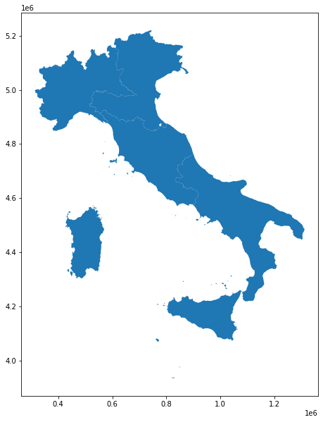
you can plot it
macroregions.plot(figsize=(10,10))
<matplotlib.axes._subplots.AxesSubplot at 0x7f7e85654a90>

macroregions.plot(figsize=(10,10))
plt.show()
… and new we can use the classic methods of the pandas DataFrame.
Eg.
extract a (geo)DataFrame by filter from an attribute
macroregions.DEN_RIP
0    Nord-Ovest
1      Nord-Est
2        Centro
3           Sud
4         Isole
Name: DEN_RIP, dtype: object
macroregions.DEN_RIP.unique()
array(['Nord-Ovest', 'Nord-Est', 'Centro', 'Sud', 'Isole'], dtype=object)
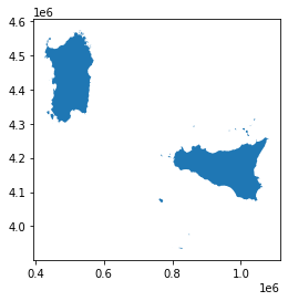
islands = macroregions[macroregions['DEN_RIP'] == 'Isole']
islands.plot()
plt.show()
macroregions.geom_type
0    MultiPolygon
1    MultiPolygon
2    MultiPolygon
3    MultiPolygon
4    MultiPolygon
dtype: object
in an ESRI shapefile the kind of geometry is always the same, but a geodataframe can accept mixed geometries for each row.
in our case we have a MultiPolygon the geometries allowed are:
| geometry | images |
|---|---|
| POINT | |
| LINESTRING | |
| LINEARRING |  |
| POLYGON | |
| MULTIPOINT | |
| MULITLINESTRING | |
| MULTIPOLYGON | |
| GEOMETRYCOLLECTION |
note: table based on the wikipedia page WKT
now we are ready to look how are the geometries
macroregions.geometry[0]

macroregions.DEN_RIP[0]
'Nord-Ovest'
macroregions.geometry[1]

macroregions.DEN_RIP[1]
'Nord-Est'
macroregions.geometry[2]

macroregions.DEN_RIP[2]
'Centro'
macroregions.geometry[3]

macroregions.DEN_RIP[3]
'Sud'
macroregions.geometry[4]

macroregions.DEN_RIP[4]
'Isole'
the red color, in this case, means a mistake on the geometries!!!
… and we can check it!
macroregions.geometry.is_valid
0     True
1     True
2     True
3    False
4    False
dtype: bool
a tip to try to correct it
macroregions.geometry[4].buffer(0)

Do you want know the centroid position of each geometry?
macroregions.geometry.centroid
0     POINT (478144.288 5011450.461)
1     POINT (702031.574 5039727.063)
2     POINT (756687.164 4757581.199)
3    POINT (1061529.198 4529724.362)
4     POINT (736519.273 4300285.997)
dtype: geometry
the output of the geometries is in well knowtext format (WKT)
but … how are expressed the coordinates?? we have to know the Coordinate Reference System (CRS)
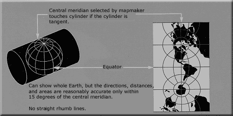
SPATIAL PROJECTIONS
CRS = Coordinate Reference System
The Earth isn’t FLAT
The true size

https://thetruesize.com/
How to convert in latitude/longitude?
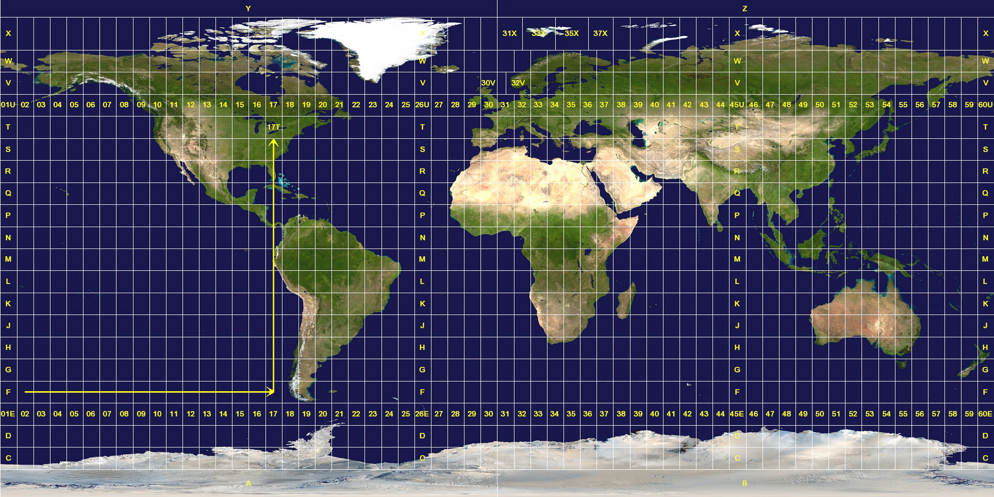
macroregions.crs
<Projected CRS: EPSG:32632>
Name: WGS 84 / UTM zone 32N
Axis Info [cartesian]:
- E[east]: Easting (metre)
- N[north]: Northing (metre)
Area of Use:
- name: Between 6°E and 12°E, northern hemisphere between equator and 84°N, onshore and offshore. Algeria. Austria. Cameroon. Denmark. Equatorial Guinea. France. Gabon. Germany. Italy. Libya. Liechtenstein. Monaco. Netherlands. Niger. Nigeria. Norway. Sao Tome and Principe. Svalbard. Sweden. Switzerland. Tunisia. Vatican City State.
- bounds: (6.0, 0.0, 12.0, 84.0)
Coordinate Operation:
- name: UTM zone 32N
- method: Transverse Mercator
Datum: World Geodetic System 1984 ensemble
- Ellipsoid: WGS 84
- Prime Meridian: Greenwich
EPSG?
European Petroleum Survey Group (1986-2005)
IOGP - International Association of Oil & Gas Producers (2005-now)
An important project is the EPSG registry - the dataset of geodetic parameters

macroregions.geometry.centroid.to_crs(epsg=4326)
0     POINT (8.72145 45.25621)
1    POINT (11.58513 45.48181)
2    POINT (12.14541 42.92765)
3    POINT (15.64719 40.72671)
4    POINT (11.72430 38.81962)
dtype: geometry
macroregions.to_crs(epsg=4326).geometry[1]

macroregions.geometry[1]

WGS84 VS ETRS89
| WGS84 | ETRS89 |
|---|---|
 |
 |
exploring a .prj file
f=open('RipGeo01012022_WGS84.prj','r')
f.read()
'PROJCS["WGS_1984_UTM_Zone_32N",GEOGCS["GCS_WGS_1984",DATUM["D_WGS_1984",SPHEROID["WGS_1984",6378137.0,298.257223563]],PRIMEM["Greenwich",0.0],UNIT["Degree",0.0174532925199433]],PROJECTION["Transverse_Mercator"],PARAMETER["False_Easting",500000.0],PARAMETER["False_Northing",0.0],PARAMETER["Central_Meridian",9.0],PARAMETER["Scale_Factor",0.9996],PARAMETER["Latitude_Of_Origin",0.0],UNIT["Meter",1.0]]'
… like here
here a “pretty” version
- A `GeoDataFrame` allows to perform typical tabular data analysis together with spatial operations
- A `GeoDataFrame` (or *Feature Collection*) consists of:
- **Geometries** or **features**: the spatial objects
- **Attributes** or **properties**: columns with information about each spatial object
save the geodataframe
macroregions.to_crs(epsg=4326).to_file('macro_regions.geojson',driver='GeoJSON')
- the library *fiona* offers different kind of output formats
import fiona
fiona.supported_drivers
{'ARCGEN': 'r',
 'DXF': 'rw',
 'CSV': 'raw',
 'OpenFileGDB': 'r',
 'ESRIJSON': 'r',
 'ESRI Shapefile': 'raw',
 'FlatGeobuf': 'rw',
 'GeoJSON': 'raw',
 'GeoJSONSeq': 'rw',
 'GPKG': 'raw',
 'GML': 'rw',
 'OGR_GMT': 'rw',
 'GPX': 'rw',
 'GPSTrackMaker': 'rw',
 'Idrisi': 'r',
 'MapInfo File': 'raw',
 'DGN': 'raw',
 'OGR_PDS': 'r',
 'S57': 'r',
 'SQLite': 'raw',
 'TopoJSON': 'r',
 'libkml': 'rw',
 'LIBKML': 'rw'}
enable the support for the KML format
fiona.drvsupport.supported_drivers['libkml'] = 'rw' # enable KML support which is disabled by default
fiona.drvsupport.supported_drivers['LIBKML'] = 'rw' # enable KML support which is disabled by default
download file from colab
… otherwise you can simply load the file from your filesystem where you hosted this script :)
#uncomment the next lines if you want download the file from google colab
# from google.colab import files
#files.download('macro_regions.geojson')
… and visualize it on http://geojson.io

Other Examples
Explore Natural Earth Data
![]()
https://www.naturalearthdata.com/
url_dispusted_areas = "https://www.naturalearthdata.com/http//www.naturalearthdata.com/download/10m/cultural/ne_10m_admin_0_disputed_areas.zip"
Exercise
- load the shapefile of ISTAT with the information of the provinces
- filter it for an italian provice at your choice (eg. Trento)
- plot it
- load the shapefile of ISTAT with the informations of the muncipalities
- identify the cities of the province selected with the biggest and smallest area
- extract all the centroids of the areas expressed in WGS84
- select all the muncipalities of the Province of Trento
- extract a representative point for the area of each municipality converted in WGS84
suggestion: .representative_point() - save the points in a GeoJSON file
- calculate the distance on the geodentic between the municipality with the big area and smallest area by using the centroid
- download the shapefile of the lakes and bodies of water of Trentino - projection Monte Mario zone 1
- plot the geometries where Fktuso is “02”
- convert in WGS84 and create a geojson