Lesson 05

Street Network Analysis

based on osnmx and pandana goals of the tutorial

• basic concepts of network analysis
• routing
• bearing

based on the open data of:

• OpenStreetMap

requirements

• python knowledge
• geopandas
• openstreetmap

status
“My Way”

---

Setup

for this tutorial we will use OSMnx = (openstreetmap + networkx)

Boeing, G. 2017. “OSMnx: New Methods for Acquiring, Constructing, Analyzing, and Visualizing Complex Street Networks.” Computers, Environment and Urban Systems 65, 126-139. doi:10.1016/j.compenvurbsys.2017.05.004

try:
    import pygeos
except ModuleNotFoundError as e:
    !pip install pygeos==0.13
    import pygeos

… and now we can install OSMnx

try:
    import osmnx  as ox
except ModuleNotFoundError as e:
    !pip install osmnx==1.2.2
      import osmnx  as ox
if ox.__version__ != "1.2.2":
    !pip install -U osmnx==1.2.2
    import osmnx  as ox

… and all the other packages needed for this lesson

try:
    import mapclassify
except ModuleNotFoundError as e:
    !pip install mapclassify
    import mapclassify

if mapclassify.__version__ != "2.4.3":
  !pip install -U mapclassify==2.4.3

try:
    import pyrosm
except ModuleNotFoundError as e:
    !pip install pyrosm==0.6.1
    import pyrosm

import geopandas as gpd
import warnings
warnings.filterwarnings("ignore") 

Let’s start with OSMnx

import osmnx as ox
import matplotlib.pyplot as plt

prepare the data

… we can choose the same city used on the last tutorial

Venice in Italy

place_name = "Venezia, Lido, Venice, Venezia, Veneto, Italy"

.. and we can extract all the streets where it’s possible to drive

OSMnx creates a overpass query to ask the data inside the area of name of the city and collect all the highways where a car can move

Eg.
https://overpass-turbo.eu/s/1nnv

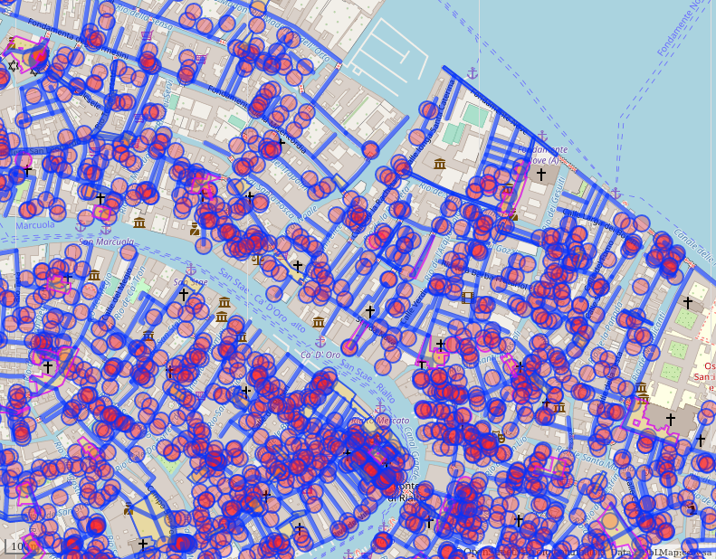
G = ox.graph_from_place(place_name, network_type='all')

OSMnx transform the data from OpenStreetMap in graph for networkx

Graph Theory

text from wikipedia

A graph is made up of vertices (also called nodes or points) which are connected by edges (also called links or lines)

A distinction is made between undirected graphs, where edges link two vertices symmetrically, and directed graphs, where edges link two vertices asymmetrically;

Example
undirected graph with three nodes and three edges.

Example
a directed graph with three vertices and four directed edges
(the double arrow represents an edge in each direction).

the type of graph generated by OSMnx is a MultiDiGraph: a directed graphs with self loops and parallel edges

more information here

type(G)

networkx.classes.multidigraph.MultiDiGraph

OSMnx converts the graph from latitude/longitude (WGS83) to the right UTM coordinate reference system for the area selected

G_proj = ox.project_graph(G)

from osmnx you can create geodataframes (gdfs) from a netxworkx Graph

gdfs = ox.graph_to_gdfs(G_proj)

type(gdfs)

tuple

0 => nodes (points)
1 => edges (lines)

type(gdfs[0])

geopandas.geodataframe.GeoDataFrame

gdfs[0].geometry.type.unique()

array(['Point'], dtype=object)

gdfs[1].geometry.type.unique()

array(['LineString'], dtype=object)

gdfs[1].crs

<Derived Projected CRS: +proj=utm +zone=33 +ellps=WGS84 +datum=WGS84 +unit ...>
Name: unknown
Axis Info [cartesian]:
- E[east]: Easting (metre)
- N[north]: Northing (metre)
Area of Use:
- undefined
Coordinate Operation:
- name: UTM zone 33N
- method: Transverse Mercator
Datum: World Geodetic System 1984
- Ellipsoid: WGS 84
- Prime Meridian: Greenwich

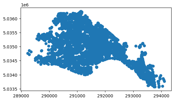
extract only the nodes (projected)

nodes_proj = ox.graph_to_gdfs(G_proj, edges=False, nodes=True)

type(nodes_proj)

geopandas.geodataframe.GeoDataFrame

nodes_proj.crs

<Derived Projected CRS: +proj=utm +zone=33 +ellps=WGS84 +datum=WGS84 +unit ...>
Name: unknown
Axis Info [cartesian]:
- E[east]: Easting (metre)
- N[north]: Northing (metre)
Area of Use:
- undefined
Coordinate Operation:
- name: UTM zone 33N
- method: Transverse Mercator
Datum: World Geodetic System 1984
- Ellipsoid: WGS 84
- Prime Meridian: Greenwich

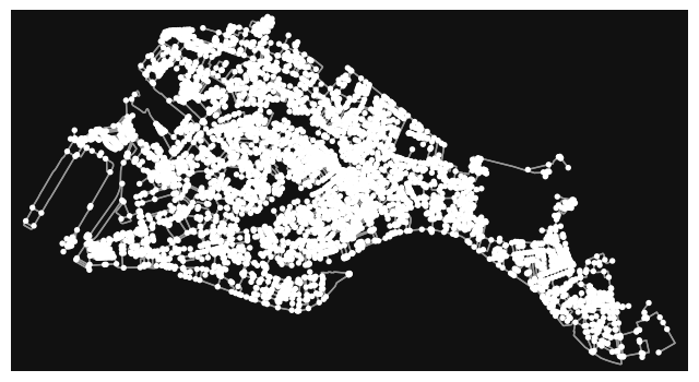
nodes_proj.plot()
plt.show()

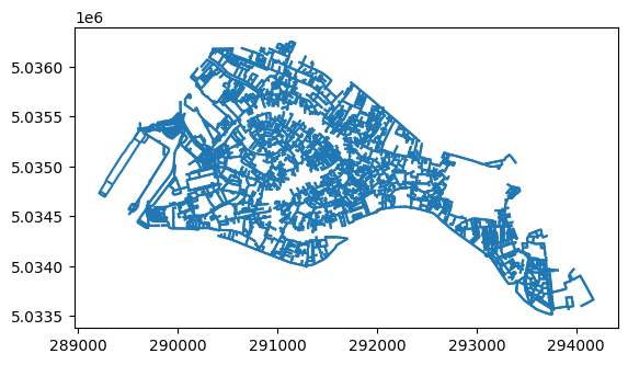
lines_proj = ox.graph_to_gdfs(G_proj, nodes=False)

lines_proj.plot()
plt.show()

… and we can use it as a normal geodaframe

Eg:
what sized area does our network cover in square meters?

nodes_proj.unary_union.convex_hull

graph_area_m = nodes_proj.unary_union.convex_hull.area
graph_area_m

7679268.778717262

with OSMnx we can extract some basic statistics

ox.basic_stats(G_proj, area=graph_area_m, clean_int_tol=15)

{'n': 5020,
 'm': 12539,
 'k_avg': 4.995617529880478,
 'edge_length_total': 366879.9689999989,
 'edge_length_avg': 29.25910909960913,
 'streets_per_node_avg': 2.54003984063745,
 'streets_per_node_counts': {0: 0,
  1: 1359,
  2: 5,
  3: 3259,
  4: 382,
  5: 14,
  6: 0,
  7: 1},
 'streets_per_node_proportions': {0: 0.0,
  1: 0.2707171314741036,
  2: 0.00099601593625498,
  3: 0.649203187250996,
  4: 0.07609561752988048,
  5: 0.0027888446215139444,
  6: 0.0,
  7: 0.00019920318725099602},
 'intersection_count': 3661,
 'street_length_total': 186643.2119999999,
 'street_segment_count': 6355,
 'street_length_avg': 29.36950621557827,
 'circuity_avg': 1.0612066989278592,
 'self_loop_proportion': 0.0033044846577498033,
 'clean_intersection_count': 718,
 'node_density_km': 653.7080736010566,
 'intersection_density_km': 476.7380990943164,
 'edge_density_km': 47775.378043387376,
 'street_density_km': 24304.81565084334,
 'clean_intersection_density_km': 93.49848542740213}

stats documentation: https://osmnx.readthedocs.io/en/stable/osmnx.html#module-osmnx.stats

Glossary of the terms used by the statistics

For a complete list look the networkx documentation

• density
  defines the density of a graph. The density is 0 for a graph without edges and 1 for a complete graph. The density of multigraphs can be higher than 1.
• center
  is the set of points with eccentricity equal to radius.
• betwnees centrality
  is the number of possible interactions between two non-adjacent points
• closeness centrality
  is the average distance of a point from all the others
• clustering coefficient
  the measure of the degree to which points in a graph tend to cluster together
• degree centrality
  the number of lines incident upon a point
• eccentricity
  the eccentricity of a point in a graph is defined as the length of a longest shortest path starting at that point
• diameter
  the maximum eccentricity
• edge connectivity
  is equal to the minimum number of edges that must be removed to disconnect a graph or render it trivial.
• node connectivity
  is equal to the minimum number of points that must be removed to disconnect a graph or render it trivial.
• pagerank
  computes a ranking of the nodes (points) in a graph based on the structure of the incoming links (lines). It was originally designed as an algorithm to rank web pages.
• periphery
  is the set of nodes with eccentricity equal to the diameter
• radius
  is the minimum eccentricity.

… and we can plot the map

fig, ax = ox.plot_graph(G)
plt.show()

import networkx as nx

# convert graph to line graph so edges become nodes and vice versa
edge_centrality = nx.closeness_centrality(nx.line_graph(G))
nx.set_edge_attributes(G, edge_centrality, 'edge_centrality')

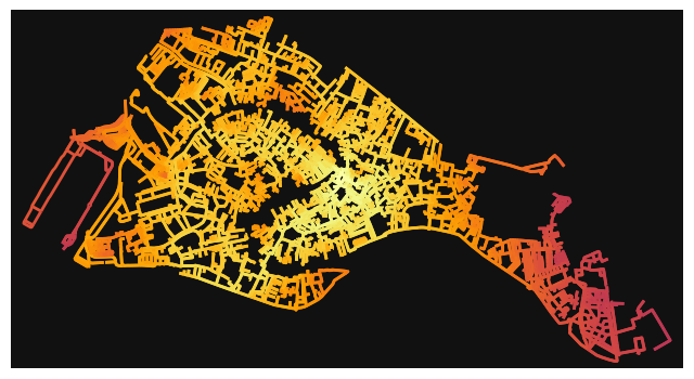
# color edges in original graph with closeness centralities from line graph
ec = ox.plot.get_edge_colors_by_attr(G, 'edge_centrality', cmap='inferno')
fig, ax = ox.plot_graph(G, edge_color=ec, edge_linewidth=2, node_size=0)
plt.show()

Find the shortest path between 2 points by minimizing travel time

calculate the travel time for each edge

define the origin and destination

Example:

from the train station of Venezia Santa Lucia to the Rialto Bridge

train station

Venezia Santa Lucia

lat: 45.4410753
lon: 12.3210322

Rialto Bridge

Ponte di Rialto

lat: 45.43805
lon: 12.33593

find the node on the graph nearest on the point given

thes two points are NOT on the graph.

We need to find the nodes nearest

point_nearest_train_station = ox.distance.nearest_nodes(G,Y=45.4410753,X=12.3210322)
point_nearest_bridge_rialto = ox.distance.nearest_nodes(G,Y=45.43805,X=12.33593)

# impute missing edge speeds and calculate edge travel times with the speed module
G = ox.speed.add_edge_speeds(G)
G = ox.speed.add_edge_travel_times(G)

calculate the time to walk over each edges

G = ox.graph_from_place(place_name, network_type='walk')

plot the walkable street network

fig, ax = ox.plot_graph(G)
plt.show()

G = ox.add_edge_speeds(G)
G = ox.add_edge_travel_times(G)

… geopandas investigation

edges = ox.graph_to_gdfs(G,edges=True,nodes=False)

edges.head(3)

			osmid	bridge	name	highway	oneway	reversed	length	speed_kph	travel_time	width	geometry	tunnel	lanes	maxspeed	est_width	access	area	service	junction
u	v	key
27178184	764403528	0	166489461	yes	Ponte di Rialto	footway	False	False	9.935	39.6	0.9	NaN	LINESTRING (12.33569 45.43820, 12.33561 45.43813)	NaN	NaN	NaN	NaN	NaN	NaN	NaN	NaN
	1675825096	0	166489461	yes	Ponte di Rialto	footway	False	True	5.120	39.6	0.5	NaN	LINESTRING (12.33569 45.43820, 12.33573 45.43823)	NaN	NaN	NaN	NaN	NaN	NaN	NaN	NaN
	8670969688	0	450089474	yes	Ponte di Rialto	steps	False	False	9.212	39.6	0.8	7	LINESTRING (12.33569 45.43820, 12.33560 45.43825)	NaN	NaN	NaN	NaN	NaN	NaN	NaN	NaN

edges.columns

Index(['osmid', 'bridge', 'name', 'highway', 'oneway', 'reversed', 'length',
       'speed_kph', 'travel_time', 'width', 'geometry', 'tunnel', 'lanes',
       'maxspeed', 'est_width', 'access', 'area', 'service', 'junction'],
      dtype='object')

edges[edges.travel_time == edges.travel_time.max()].name

u           v           key
1927219469  4068932557  0      NaN
4068932557  1927219469  0      NaN
Name: name, dtype: object

edges[edges.travel_time == edges.travel_time.max()].osmid

u           v           key
1927219469  4068932557  0      [404610512, 404610513]
4068932557  1927219469  0      [404610512, 404610513]
Name: osmid, dtype: object

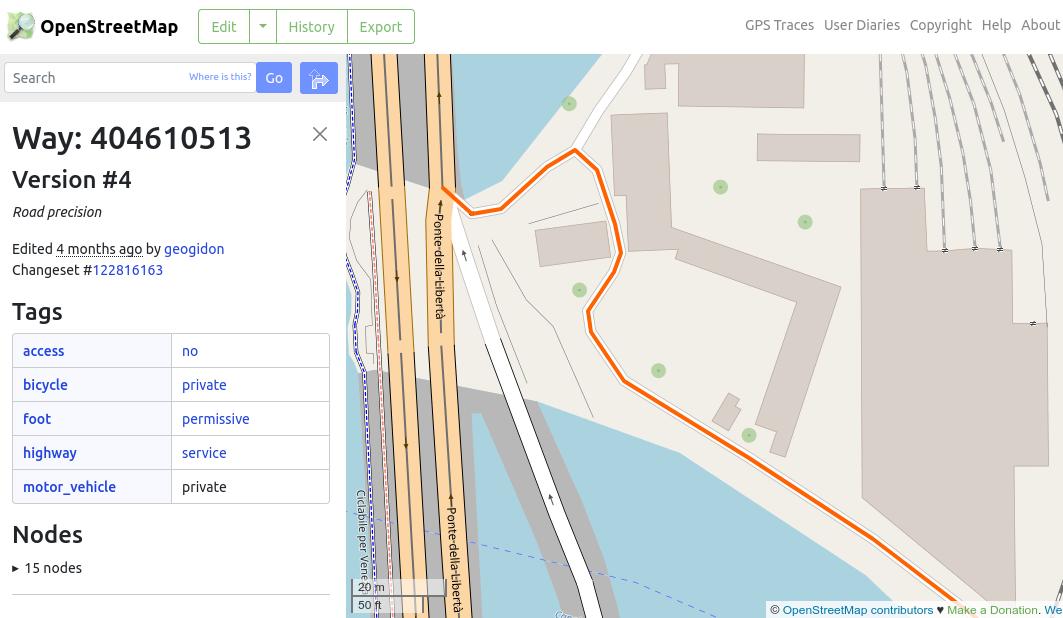
https://www.openstreetmap.org/way/404610513

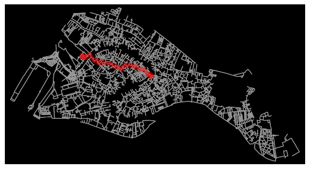
find the shortest path between the train station and Rialto bridge

# find the shortest path between nodes, minimizing travel time, then plot it
route = ox.shortest_path(G, point_nearest_train_station, point_nearest_bridge_rialto, weight="travel_time")

route

[1927219479,
 3527986497,
 2493856508,
 9055796707,
 1921651801,
 27239442,
 5372700772,
 4899902714,
 1855450146,
 3371984917,
 2514483400,
 1858198295,
 1858198260,
 3371984290,
 3371984894,
 5360645772,
 1855473678,
 1855473687,
 4849873712,
 4849867342,
 1856706712,
 3389313497,
 5149979474,
 2732099927,
 4843929370,
 2732099913,
 2732099919,
 2732099909,
 2732099904,
 4803731379,
 4846061555,
 1857205293,
 1857205281,
 3392463459,
 1857205288,
 1856788519,
 3392463420,
 3392463416,
 1857148234,
 1840378080,
 2249214723,
 4803872602,
 4803871721,
 1857139330,
 4902225461,
 1857139271,
 1857139307,
 1857139318,
 1857139273,
 1857139324,
 1857139332,
 4983211717,
 4983211715,
 5649829357,
 5649829356,
 5649829355,
 4983211716,
 8670969688,
 27178184,
 5395065019]

these values are the ids of each node of the graph

G.nodes[5395065019]

{'y': 45.4380532, 'x': 12.3359319, 'street_count': 4}

nodes = ox.graph_to_gdfs(G,edges=False,nodes=True)

nodes

	y	x	street_count	highway	geometry
osmid
27178184	45.438197	12.335686	4	NaN	POINT (12.33569 45.43820)
27178422	45.432325	12.337206	4	NaN	POINT (12.33721 45.43233)
27178433	45.429240	12.327350	3	NaN	POINT (12.32735 45.42924)
27178442	45.430846	12.320432	1	NaN	POINT (12.32043 45.43085)
27223839	45.434570	12.350321	3	NaN	POINT (12.35032 45.43457)
...	...	...	...	...	...
10108266854	45.437868	12.350362	3	NaN	POINT (12.35036 45.43787)
10118200318	45.431717	12.358683	3	NaN	POINT (12.35868 45.43172)
10118200319	45.431700	12.358617	3	NaN	POINT (12.35862 45.43170)
10118200325	45.431011	12.354432	3	NaN	POINT (12.35443 45.43101)
10118200326	45.430948	12.354443	1	NaN	POINT (12.35444 45.43095)

5016 rows × 5 columns

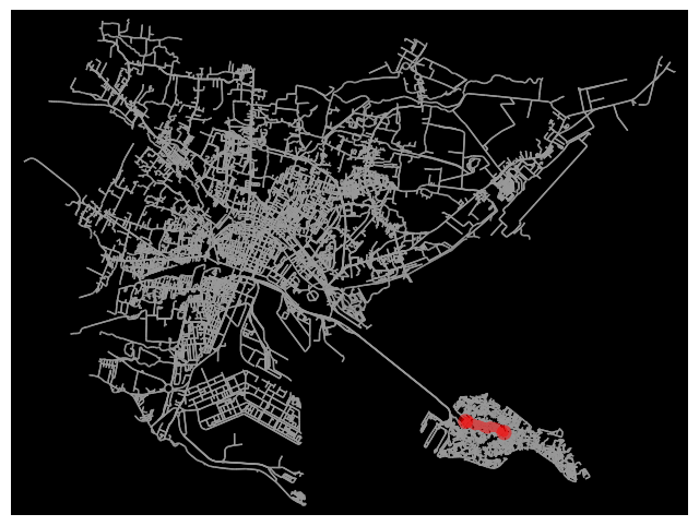
fig, ax = ox.plot_graph_route(G, route, route_linewidth=6, node_size=0, bgcolor='k')
plt.show()

ox.plot_route_folium(G,route,popup_attribute='name',tiles='CartoDB dark_matter')
#OpenStreetMap
#Stamen Terrain
#Steman Toner
#Stamen Watercolor
#CartoDB positron
#CartoDB dark_matter

Make this Notebook Trusted to load map: File -> Trust Notebook

how long is our route in meters?

edge_lengths = ox.utils_graph.get_route_edge_attributes(G, route, 'length')
sum(edge_lengths)

1614.4050000000004

how many minutes does it take?

import datetime

edge_times = ox.utils_graph.get_route_edge_attributes(G, route, 'travel_time')
seconds = sum(edge_times)

seconds

146.50000000000003

str(datetime.timedelta(seconds=seconds))

'0:02:26.500000'

calculate bearing

Calculate the compass bearing from origin node to destination node for each edge in the directed graph then add each bearing as a new edge attribute. Bearing represents angle in degrees (clockwise) between north and the direction from the origin node to the destination node.

cols = ['city']
names = [('Roma'),('Trento'),('Genova'),('Trieste'),('Venezia')]
cities = gpd.GeoDataFrame(names,columns=cols)
geo_cities = gpd.tools.geocode(cities.city, provider="arcgis")

cities

	city
0	Roma
1	Trento
2	Genova
3	Trieste
4	Venezia

geo_cities

	geometry	address
0	POINT (12.49565 41.90322)	Roma
1	POINT (11.11929 46.07005)	Trento
2	POINT (8.93917 44.41048)	Genova
3	POINT (13.77269 45.65757)	Trieste
4	POINT (12.31815 45.43811)	Venezia

trento = geo_cities[geo_cities.address == 'Trento'].geometry

trento.geometry.x.values[0]

11.119290000000035

roma = geo_cities[geo_cities.address == 'Roma']
genova = geo_cities[geo_cities.address == 'Genova']
trieste = geo_cities[geo_cities.address == 'Trieste']
venezia = geo_cities[geo_cities.address == 'Venezia']

#Trento - Roma
ox.bearing.calculate_bearing(trento.geometry.y.values[0],trento.geometry.x.values[0],roma.geometry.y.values[0],roma.geometry.x.values[0])

166.14931950629008

#Trento - Trieste
ox.bearing.calculate_bearing(trento.geometry.y.values[0],trento.geometry.x.values[0],trieste.geometry.y.values[0],trieste.geometry.x.values[0])

101.62965042129908

#Trento - Venezia
ox.bearing.calculate_bearing(trento.geometry.y.values[0],trento.geometry.x.values[0],venezia.geometry.y.values[0],venezia.geometry.x.values[0])

126.6391923258096

#Trento - Genova
ox.bearing.calculate_bearing(trento.geometry.y.values[0],trento.geometry.x.values[0],genova.geometry.y.values[0],genova.geometry.x.values[0])

223.54736298562963

PyORSM

Network Analysis with PyORSM + OSMnx + NetworkX

url_download_venice_pbf = 'https://osmit-estratti-test.wmcloud.org/dati/poly/comuni/pbf/027042_Venezia_poly.osm.pbf'
import urllib.request
urllib.request.urlretrieve(url_download_venice_pbf ,"venezia_osm.pbf")

('venezia_osm.pbf', <http.client.HTTPMessage at 0x7fe072903070>)

osm = pyrosm.OSM("venezia_osm.pbf") 

nodes, edges = osm.get_network(nodes=True)

NetworkX

calculate the distances between the train station and Rialto bridge

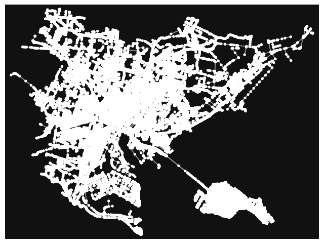
G = osm.to_graph(nodes, edges, graph_type="networkx")

ox.plot_graph(G)
plt.show()

#eg. lenght
route = ox.shortest_path(G, point_nearest_train_station, point_nearest_bridge_rialto, weight='length')
fig, ax = ox.plot_graph_route(G, route, route_linewidth=6, node_size=0, bgcolor='k')
plt.show()

note:
you can also use pandana or igraph with pyrosm

Calculate isochornes

trip_times = [3, 6, 9, 15]  # in minutes
travel_speed = 4  # walking speed in km/hour
from shapely.geometry import Point

# we select the train station as center
center_node = point_nearest_train_station
center_node = point_nearest_bridge_rialto

# add an edge attribute for time in minutes required to traverse each edge
meters_per_minute = travel_speed * 1000 / 60  # km per hour to m per minute
for orig,dest, p, data in G_proj.edges(data=True, keys=True):
    data["time"] = data["length"] / meters_per_minute

# make the isochrone polygons
isochrone_polys = []
for trip_time in sorted(trip_times, reverse=True):
    subgraph = nx.ego_graph(G_proj, center_node, radius=trip_time, distance="time")
    node_points = [Point((data["x"], data["y"])) for node, data in subgraph.nodes(data=True)]
    bounding_poly = gpd.GeoSeries(node_points).unary_union.convex_hull
    isochrone_polys.append(bounding_poly)

crs_proj = ox.graph_to_gdfs(G_proj)[0].crs

data = {'trip_time': sorted(trip_times, reverse=True), 'geometry': isochrone_polys}
isochrones = gpd.GeoDataFrame(data,crs=crs_proj)

isochrones.explore(column='trip_time',cmap='Reds')

Make this Notebook Trusted to load map: File -> Trust Notebook

---

Exercise

• identify the shortest path by walk to reach the Castle of Trento from the main train station of Trento
• identify the streets network orientation of the cities: Trento-Italy, Verona-Italy, Munich-Germany, Athens-Greece
• locate the student residences of Trento in OpenStreetMap and identify services in an area of 15 minutes based on the concept of Carlos Moreno of the 15 minute city
  “…a way to ensure that urban residents can fulfill six essential functions within a 15-minute walk [or bike] from their dwellings: living, working, commerce, healthcare, education and entertainment…”

You are free to use OSMnx, Pyrosm with networkx or pandana or igraph